1  Purpose

• To experimentally determine the speed of signal propagation and the characteristic impedance of transmission lines.

• To interpret these measurements in terms of the capacitance and inductance per unit length of the cable.

• To observe termination effects in cables and interpret them in terms of virtual running waves.

• To observe clipping, capacitive charging and resonance in cables and interpret the observations in terms of the previously measured characteristics.

2  Procedure

At low frequencies we can approximate the wires and cables that are used to connect the separate elements of the circuit as ideal connectors which transmit voltage and current unchanged in magnitude. However, in high frequencies ( ~  1 MHz.) and in pulse applications, this approximation breaks down and the cable itself must be considered as an integral part of the circuit with its own characteristic properties.

The line you will use for these measurements is a coil of coaxial cable (RG-58 or a similar RG-223/U whish is a double shielded version of the same Z₀ and u₀). The length of the cable (l) is indicated on the attached tag. Two of the measurable parameters associated with the line are:

First use the coaxial cable to connect the Pulse Generator output to the scope input (say to ``CH 1'').

1. Adjust the pulse generator to emit an pulse of approximate width about 30 to 100 ns (1 ns = 10^-9 sec).
2. Adjust the scope sensitivity, time/cm and trigger so you can verify the pulse width.

Now make the following circuit to study the reflected pulses and measure the cable attributes.

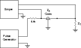
Figure 1:

1. Uncouple the cable you have just used.
2. Attach a BNC ``Tee'' to the scope and connect the first end of the cable to one end of the ``Tee''.
3. Attach a small shielded box which has, within, a ~ 5.6k resistor, to the pulse generator using a short cable. It is very important in constructing the circuit that the signals be shielded as much as possible and that the leads be as short as possible. This minimizes the noise pick-up and is a general rule to be observed at all times in the laboratory.

4. Using another BNC ``Tee'', attach the second end of the cable to the other side of the 5.6k resistor box and connect this end to the other scope channel.

5. Verify that your circuit will bring the signal from the pulse generator and feed it through the 5.6k resistor and though the cable to the scope input.

6. Ensure that the pulses are well separated. In other words, ensure that the the pulse period or time between pulses is large compared with the pulse width.

7. The high impedance input at the scope and 5.6k resistor lead to repeated reflections of the pulses at the two ends of the cable.
8. With the scope, examine the pulse on the near end with the far end open (Z_T = ¥) and shorted (Z_T = 0). In the open ended case, you may be interested in examining the signal at the far end on the second scope channel.
9. Interpret your observations.
10. Measure, as carefully as you can, the length of time required for the signal to make 10-20 round trips on the cable. Using the length of the cable, calculate the speed of propagation u₀ of the signal. Remember that, between any repeated shape upon the scope, the signal must travel twice the length of the cable!
11. To measure Z₀, the characteristic impedance of the cable, connect a variable resistor (not wire wound) to the far end of your cable and vary it until you obtain no reflection. Because of stray capacitance, you may see a small differentiated signal. Try to minimize the algebraic average of the residual signal.
12. Then with the digital VOM, measure the value of the resistance, which is then Z₀.

13. From these measurements determine the inductance per meter and the capacitance per meter using the relations:

    u0 = 1.   ____ ÖLLCL

    and

    Z0 =   æ Ö LL CL

14. Qualitatively describe the reflections obtained by varying the termination resistor from R_T = 0 to R_T = ¥.

15. Next terminate the far end with a capacitor of C ~ 500 pf and insert an incident pulse of width T » ¹/₂t, where t is the round trip time.

16. For the capacitor termination determine which features of the pulse are related by Fourier transformation to high and low frequencies and analyze how these extreme frequencies ``see'' the capacitor. (Or think of the impedance of the capacitor when the voltage across it is changing rapidly or slowly.)

17. Next feed a pulse T >> 100 t into the cable (still through the 5K resistor); and observe the results at the near end with the far end open. This shows the superposition of running waves each delayed a time t with respect to one another and all in phase. The result is that you see a ``stairstep'' wave which corresponds to the capacitive charging of your transmission line. It is clear that the effective capacitance is C_eff = lC_L, where l is the length of the cable.

    Draw the equivalent circuit showing component values and calculate the RC time constant of the exponential charging.

18. Measure the time constant (of the ``discharge'', so you have a well defined asymptote at zero) and verify your expectation.

    The results obtained with the far end shorted illustrate the use of ``shorting stubs''.

19. Now short the far end and terminate the near end with Z₀. This illustrates the use of ``shorting stubs'' in pulse shaping. For input pulses of any width we get an output pulse of width 2l/u₀ where l is the length of the shorted cable, which can be chosen at will. The negative going portion of the wave can be removed in practical situations with a diode clamp.

20. If time permits, eliminate the 5k resistor and feed the signal directly into the cable. Note and explain the differences from your previous observations.