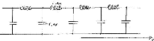
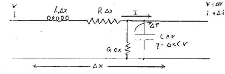
Consider one such cell corresponding to the components between position x and position x+Dx along the transmission line.
Similarly a twisted pair transmission line has two conducting rods or wires which slowly wind around each other. A cross section made at any distance along the line is the same as a cross section made at any other point on the line.
We want to understand the voltage - Current relationships of transmission lines.
Define L to be the inductance/unit length and C to be the capacitance/unit length.
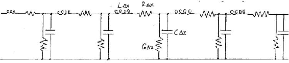
Consider a transmission line to be a pair of conductors divided into a number of cells with each cell having a small inductance in one line and having small capacitance to the other line.
In the limit of these cells being very small, they can represent a distributed inductance with distributed capacitance to the other conductor.
Consider one such cell corresponding to the components between position x
and position x+Dx along the
transmission line.
The small series inductance is L.Dx
and the small parallel capacitance is C.Dx.
Define the voltage and current to the right on the left side to be V and I. Define the voltage and current to the right on the right side to be V+DV and I+DI.
We now can get two equations.
The charge on the cell's capacitance = capacitance x voltage = C.Dx.V and so the current leaving the capacitance to provide DI must be;
DI = -[(ļ)/( ļt)](Charge) = -[(ļ)/( ļt)](C.Dx.V)
The minus sign is due to the current leaving the capacitor.
DI = -C.Dx. [(ļV)/( ļt)]
[(DI)/( Dx)] = - C.[(ļV)/( ļt)]
Note the minus sign.
The voltage increment DV between the left and right ends of the cell is due to the changing current through the cell's inductance. (Lenz's Law)
DV = - Inductance . [(ļI)/( ļt)] = - Dx .L. [(ļI)/( ļt)]
[(DV)/( Dx)] = - L.[(ļI)/( ļt)].
Now take the limit of the cell being made very small so that the inductance and capacitance are uniformly distributed. The two equations then become
[(ļI)/( ļx)] = - C.[(ļV)/( ļt)] Equation 1.
[(ļV)/( ļx)] = - L.[(ļI)/( ļt)] Equation 2.
Remember that L and C are the inductance/unit length measured, in Henries/meter and are the capacitance/unit length measured in Farads/meter.
Differentiate equation 2 with respect to the distance x.
[(ļ)/( ļx)]([(ļV)/( ļx)]) = - L. [(ļ)/( ļx)]([(ļI)/( ļt)])
[(ļ2V)/( ļx2)] = -L. [(ļ)/( ļx)]([(ļI)/( ļt)])
x and t are independent variables and so the order of the partials can be changed.
[(ļ2V)/( ļx2)] = -L. [(ļ)/( ļt)]([(ļI)/( ļx)])
Now substitute for [(ļI)/( ļx)] from equation 1 above
[(ļ2V)/( ļx2)] = -L. [(ļ)/( ļt)](-C.[(ļV)/( ļt)])
[(ļ2V)/( ļx2)] = LC. [(ļ2 V)/( ļt2)] Equation 3
This is usually called the Transmission Line Differential Equation.
Notes
The Transmission Line Differential Equation 3 above does NOT have a minus sign.
The Transmission Line Differential Equation 3 above is a normal 1 dimensional wave equation and is very similar to other wave equations in physics. From experience with such wave equations, we can try the normal solution of the form
V = V(s)
where s is a new variable s = x+ut. Substituting this into the two sides of the Transmission Line Differential Equation 3 above we get the two sides being
[(ļ2V)/( ļx2)] and [1/( u2)]. [(ļ2 V)/( ļt2)]
Thus the form V(x+ut) can satisfy the Transmission Line Differential Equation 3 if and only if
[1/( u2)] = LC Equation 4.
Both roots of this satisfy the Equation 3.
u = ą[1/( [ÖLC])]
The two roots give slightly different solutions and so, since the equation 3 is linear, any linear combination of the two solutions is a valid solution. Define u as the positive root
V = f(x-ut) + g(x+ut) Equation 6.
Where f() and g() are arbitrary single valued functions which can be very different.
g(x+ut) describes a wave propagating with no change in shape towards x = -Ĩ.
V = V(x-ut)
From this we can show, by differentiating, that:
-u[(ļV)/( ļx)] = [(ļV)/( ļt)]
[(ļV)/( ļx)] = -1/u.[(ļV)/( ļt)] Equation 7.
Also from equation 2. above
[(ļV)/( ļx)] = - L.[(ļI)/( ļt)] Equation 2.
Equation 2 and equation 7 will have a common solution only if the two right hand sides are the same
1/u.[(ļV)/( ļt)] = L.[(ļI)/( ļt)]
V = uL.I
This can be rewritten using u = [1/( [ÖLC])] from equation 5.
V = Ö{L/C}.I
and
V/I = Ö{L/C}
and the current I of the forward wave is
I = V/ Ö{L/C}
and, similarly for the backward wave
V = -Ö{L/C}.I
V/I = -Ö{L/C}
and the current I of the backward wave is
I = -V/ Ö{L/C}
Thus the general solution for both waves for the current I is
I = (f(x-ut)-g(x+ut))/ Ö{L/C} Equation 7
which can be compared with the earlier equation for the voltage
V = f(x-ut) + g(x+ut) Equation 6.
Z0 = |[Voltage/ Current]| = |V/I| = |Ö{L/C}|
For the backward wave:
Z0 = |[Voltage/ Current]| = |V/I| = |Ö{L/C}|
With this definition of Z0 the voltage and current equations can be written:
V = f(x-ut) + g(x+ut) Equation 6.
I = [(f(x-ut))/( Z0)] - [(g(x+ut))/( Z0)] Equation 8.
The Inductance per unit length L and Capacitance per unit length C can be calculated from Electromagnetic Theory. The formulae depend upon the cross sectional shape of the conductors.
C = [(2pe)/( ln(b/a))] and
L = [(m)/( 2p)]ln(b/a).

From these, u and Z0 can be obtained
u = [1/( Ö{me})] and
Z0 = Ö{L/C} = Ö{[(m)/( 4p2e)]}ln(b/a) ģ [60/( er)]ln(b/a)
For a vacuum, of course,
uvac = [1/( Ö{m0e0})] = Velocity of light and
for polyethylene, er is about 4, and the speed is halved
upolyethylene = [Velocity of light/ 2]
Parallel Cylinders
EM theory says that a pair of parallel conducting cylinders, rods or wires,
with rod radius r and center to center separation D have
C = [(pe)/( ln(D/r))]
L = [(m)/( p)]ln(D/r)
From these, u and Z0 can be obtained
u = [1/( Ö{me})] and
Z0 = Ö{L/C} = Ö{[(m)/( 4p2e)]}ln(D/r) ģ [240/( er)]ln(D/r)
in both cases, the speed and the Characteristic Impedance depend upon logarithms of the ratio of two distances in the cross.
For most lines it is not practical to vary the ratios b/a and D/r much more than about 2.0/1 up to 10/1. Since the ln(2/1) ģ 0.69 and ln([10/ 1]) ģ 2.3 the range of impedances is normally within a moderate range (about 20 ohm to 200 ohm).
u = [1/( [ÖLC])] and Z0 = Ö{L/C}
By multiplying and dividing these equations, we can get L and C
L = [(Z0)/ u] and C = [1/( Z0u)]
For the values assumed for Z0 and u
L = [50 ohm/( 1.5×10⁸ m/s)] = 3.333×10⁻⁷ Henry/meter = 333×10-9 Henry/meter = 333 nanoHenry/meter
C = [1/( 50 ohm ×1.5×108 m/s)] = [1/( 75×108)] Farad/m = 1.333 ×10¹⁰ Farad/m = 133.3 pF/m
Thus a foot of RG58 cable with Z=50 ohm and u=half of light
has a capacitance of
ģ 0.305 m/ft×1.333 pF/m = 40 pF.
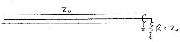
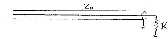
Consider a transmission line which is terminated by a resistor, to ground,
with resistance R which is equal to to characteristic
impedance Z0. A signal is introduced by a module to the left
(at negative x).
The general solution for V and I, from before, is
I = (f(x-ut)-g(x+ut))/ Z0 Equation 7
V = f(x-ut) + g(x+ut) Equation 6.
At x = 0 the V and I must obey these 2 equations and ALSO obey the equation (Ohm's Law) for the resistor.
V = IR = IZ0
These can only be consistent if the functions g() =0 so that
I = (f(x-ut))/ Z0
V = f(x-ut)
Thus, while there can be a forward wave, there cannot be a backward wave. Thus and forward wave cannot produce a backward wave. There are NO REFLECTIONS.
This example with a resistor R = Z0 is sometimes called using parallel termination.
Now consider a similar signal introduced from the left but with a general
value of R instead of requiring R = Z0.
V = f+g
I = [f/( Z0)]-[g/( Z0)]
If V = IR then
V = f+g = ([f/( Z0)]-[g/( Z0)]).R
f+g = f[R/( Z0)]-g[R/( Z0)]
f(1-[R/( Z0)]) = -g(1+[R/( Z0)])
g = f.([(R-Z0)/( R+Z0)])
Thus the forward wave causes a backward wave.
The backward wave is, in general, smaller and we call
 = g/f = ([(R-Z0)/( R+Z0)]) the ``voltage reflection coefficient''.
checks
 = g/f = [(100-50)/( 100+50)] = 1/3
If R = Z0, the Voltage Reflection Coefficient  = g/f = ([(R-Z0)/( R+Z0)]) = [0/ 2R] = 0 as in the previous example.
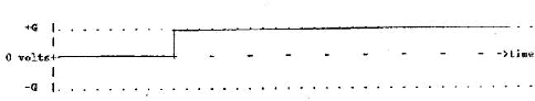
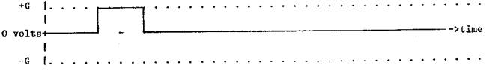
If the cable is open circuited (ie has no resistor) then R = Ĩ ohm and
using some sloppy algebra
 = g/f = ([(Ĩ-Z0)/( Ĩ+Z0)]) = [(Ĩ)/( Ĩ)] = +1
The backward wave will have the same size and shape as the incident right forward wave.
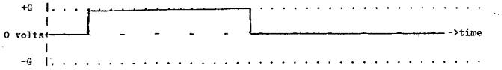
Short Circuit ``Termination'' R = 0
If the cable is short circuited (ie has zero resistance) then R = 0 ohm and
 = g/f = ([(0-Z0)/( 0+Z0)]) = (-[(Z0)/( Z0)]) = -1
The backward wave will have the same size and shape as the incident right forward wave but will be inverted.
If one cable with characteristic impedance Z1 is connected to another
long cable with characteristic impedance Z2, which is so long that signals
have not had time to reflect from the far right, then lets call the 2
functions on the left as f(x-ut) and g(x+ut). Since there is no
reflection on the right, the backward wave is absent.
Lets call the forward wave on the right as
F(x-ut) or F.
The equations for the left and right parts are
V = f+g V = F
I = [f/( Z1)]-[g/( Z1)] I = [F/( Z2)]
We must have continuity of voltage at the boundary
f+g = F when x=0
Divide this trivial equation by Z1
[f/( Z1)]+[g/( Z1)] = [F/( Z1)]
For continuity of current the currents on the two sides must be equal
[f/( Z1)]-[g/( Z1)] = [F/( Z2)]
Add the last 2 equations to eliminate g;
2[f/( Z1)] = F([1/( Z1)]+[1/( z2)]) = F[(Z2+Z1)/( Z1Z2)]
F = f[(2Z2)/( Z2+Z1)]
The factor T = [(2Z2)/( Z2+Z1)] is called the Voltage Transmission Coefficient
A challenge:
Prove that the reflected wave g here has the same formula as for the case
of a simple resistor discussed before but with the notation changed slightly
to have
the cable with characteristic impedance Z1 being terminated with
a resistor with resistance R = Z2.
Joining One Cable to three other cables.
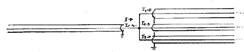
Consider one Coaxial cable joining 3 other long coaxial cables with all four
cables having the same Characteristic Impedance Z. Using the subscripts f
and g for the original and reflected voltages & currents and the subscripts
1, 2 and 3 for the voltage & current in the three other cables,
the equations to be solved are:
If-Ig = I1+I2+I3
Vf+Vg = V1 = V2 = V3
Vf = +ZIf, Vg = -ZIg,
V1 = V2 = V3 = +ZI1 = +ZI2 = +ZI3
All ``3 other long cables'' will receive a transmitted signal which is T times the original signal Vf = f(x-ut).
T = [(2Z/3)/( (Z/3+Z))] = [2Z/( Z+3Z)] = +1/2
The ``One Coaxial cable'' will receive an inverted reflection which is  times the original signal.
 = [(Z/3-Z)/( Z/3+Z)] = [(1-3)/( 1+3)] = -1/2
When does a Cable act like a Resistor?
We have seen that a transmission line acts exactly like a resistor to any circuit driving it until a reflection (the backward wave g) can return. As a typical speed of signals in cables is about 0.5 of the speed of light - a typical speed in cable of 1.5×10⁸ m/s or 150 mm/ns, the signal can propagate though a 1.5 meter cable in about 10 ns and its reflection can return 20 ns after the signal was first injected. Thus such a transmission line acts as a resistor, to any external system driving it, for about 20 ns.
How long must a cable be to act like a resistor for 1 ms?
If a transmission line acts like a resistor to any external system driving it, WHY DOES THE TRANSMISSION LINE NOT GET HOT?
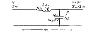
Consider charging up a 50 ohm Transmission line via a 200 ohm resistor from a battery with voltage E.
Consider the action when the switch from the battery is closed (ie connected). Assume that the signals can propagate from one end to the other in a time T.
VA = [50/( 200+50)].E = 0.2×E
Part of the signal (0.2E) reflected signal is reflected again with a voltage reflection coefficient of
 = [(200-50)/( 200+50)] = [150/ 250] = 0.6
and so a reflection of a reflection, now 0.6×0.2×E = 0.12×E, will be sent to towards the far end again.
The first example with a resistor R = Z0 is sometimes called using
parallel termination. While it has the advantage of causing reflections,
it has the disadvantage of requiring a steady current from the driving circuit
to maintain any unchanging signal. When it is important to minimize the
power spent by the driver, some folk use series resistors as shown above.
Note that we assume here that the driver has a low output impedance and the receiving module has a high input impedance.
[Be careful, the terms parallel termination and series termination are often mis-used. For example, one can buy ``series terminations for SCSI busses on computers. Although these little modules are plugged in series to the other modules on a SCSI cable, the SCSI cable carries its own grounds and supplies and the module is really a parallel termination connecting each signal line via a suitable resistor to a voltage of about +3V.]
The signal of voltage E injected on the left passes through a resistor with resistance R = Z0 before it reaches the transmission line. Thus for the first few nanoseconds, the signal on the cable is 0.5E.
This signal travels to the far end where it bounces with voltage reflection coefficient  = +1.0 and the signal received by the receiving module is 2×0.5E = E.
The reflection travels back to the near end where it ``sees'' a total resistance to ground of R = Z0. Here the voltage reflection coefficient  = 0 and no further reflections occur.
Advantage of Source Termination
- lower power load in the resistors and the drivers since there is no
current for steady DC signals.
Disadvantage of Source Termination
- if the transmission line has two or more receiving units,
then the unit near the end of the transmission line sees a single
clean transition from 0 to E. However, a unit part-way along the
transmission line will see a voltage step from 0 to 0.5E then, later,
a second voltage step from 0.5E to E.
The extra step will change the final signal shape and may confuse a number of analog signal recorders. Many digital circuits will misbehave if given an input which is half-way between logical 0 and logical 1.
Consider a sinusoidal wave form for both the forward wave and the backward wave with equal amplitudes and parameters.
V = forward + backward
V = asin[[(2px)/( l)]-wt]+asin[[(2px)/( l)]+wt]
This can be changed using SinA + Sin B = 2 Sin((A+B)/2)Cos((A-B)/2) to
V = a 2 sin[[(2px)/( l)]]cos[wt]
Note that the dependence upon position x and t has been separated and even though two signals are involved there appears to be no propagation. Also the signal at any point is simply an alternative voltage.
Signals like these can be caused by simply reflecting a sinusoidal input from an open or very high impedance at the far end, appear as standing waves. At some positions, the amplitude of the alternating voltage is zero and at other positions the amplitude of the alternating voltage can be 2a.
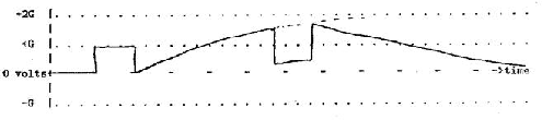
What will be the effect due to a step function wave in the cable meeting
this termination?
Define the distance x along the cable as being x = 0 at the termination and
x being negative in the actual cable.
Assume that the step function reaches the termination x = 0 at time t = 0.
We use the general solution functions we found before,
f(x-ut) to describe a wave travelling towards positive x and
g(x+ut) to describe a wave travelling towards negative x.
The voltage functions can be
V = f(x-ut) +g(x+ut)
and the corresponding current function is then
I = [(f(x-ut))/( Z0)] - [(g(x+ut))/( Z0)]
Of the two functions, we know the step function f(x-ut) but we DO NOT YET KNOW
the reflected function g(x+ut).
For the step function, the function g(x-ut is, say,
V(x-ut) = 0 when x-ut > 0 and
V(x-ut) = G when x-ut < 0.
In other words, the step signal coming from far away in the cable has the value
V = 0 then suddenly rises in a step to the value V = G when x-ut = 0.
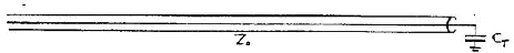
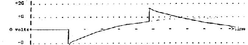
We label everything at the Termination with the subscript ``T''. At the capacitor with capacitance CT, the current combination of the step f(x-ut) travelling towards +x and its unknown reflection g(x+ut) travelling towards -x will provide a current to charge the capacitor. If VC and IC are the voltage and charging current at the capacitor, then the two equations for the voltage and current of the two travelling waves are:
VT = f+g
IT = [(f-g)/( z0)]
On the capacitor CT, the charge is QT = CTVT and the voltage rises due to the current
[(dVT)/ dt] = [1/( Z0CT)](f-g)
[(dVT)/ dt] = [1/( Z0CT)](f-(VT-f))
[(dVT)/ dt] = [1/( Z0CT)](2f-VT)
After t = 0 at x = 0, f = G and V = VT and so
[(dVT)/ dt] = -[1/( Z0CT)](VT-2G) ``differential equation''.
This has a solution for the voltage VT at the termination:
VT-2G = Ke[(-t)/( Z0CT)]
[Proof. Differentiate the tentative solution and get: [(VT)/ dt] = -[1/( Z0C)]Ke[(-t)/( Z0CT)]. Then substitute the differential equation to eliminate Ke[(-t)/( Z0CT)]. This gives [(VT)/ dt] = -[1/( Z0CT)](VT-2G) which satisfies the differential equation. ]
Find the value of K. At t = 0,
VT-2Ge0 = K
0-2G = K
VT-2G = -2Ge[(-t)/( Z0CT)]
VT = (1-e[(-t)/( Z0CT)])2G
Since V = f+g and after t = 0, we still have f = G
g = VT-G
g = (1-2e[(-t)/( Z0CT)])G
and in the general case with x < 0;
g(x+ut) = (1-2e[(-(x+ut))/( uZ0CT)])G
Using the signal speed u = Ö{[1/ LC]} and cable impedance
Z0 = Ö{L/C},
where L is the inductance per unit length,
C is the capacitance per unit length,
CT is the terminating capacitance and
G is the step of the wave travelling towards the termination,
we have uZ0 = L and so
g(x+ut) = (1-2e[(-(x+ut))/( LCT)])G
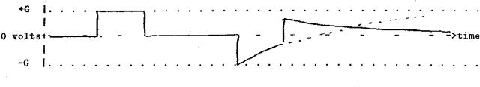
From the two items above, the reflected waveform is g(x+ut) where;
if x+ut < 0 then g(x+ut) = 0
The reflected wave due to a positive step G, starts with a negative step to -G and is followed by an exponential rise to +G. An oscilloscope at any point will see an addition of the initial step wave f(x-ut) and reflected wave g(x+ut).
The initial step wave f(x-ut) at an arbitrary x will show the trace on the scope:
The reflected wave g(x+ut) = (1-2e[(-(x+ut))/( LCT)])G
at an arbitrary x will show the trace on the scope:
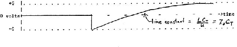
Some folk remember the shape of this reflected wave g(x+ut) by saying that
the trailing level of the step is formed from the low frequencies being in phase and these ``see'' the capacitor as an open circuit giving a trailing positive reflection.
The following examples show how the forward and backward wavefronts may be seen.
Combined signal f(x-ut)+g(x+ut) on scope:
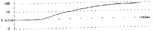
Combined signal f(x-ut)+g(x+ut) on scope:
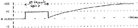
Short Pulse signal f(x-ut) on scope at large negative x:
Then if the scope is used to look at the signal closer to the termination on
the cable (still at a negative x)
due to f(x-ut) being a positive going pulse,
then the scope may show.
Combined signal f(x-ut)+g(x+ut) on scope:
The reflection g(x+ut) will look like:
then the scope will show the Combined signal f(x-ut)+g(x+ut);
Any pair of parallel conductors which have a cross and shape which are constant (independent of distance) and are far from other conductors
or any pair of parallel conductors which have a cross and shape which do not change rapidly and retain the same ratios of dimensions (independent of distance along the pair) and are far from other conductors.
If one conductor does not fully enclose the other conductor (eg twisted pair), then some of the EM field will gradually radiate away and the signal will show a steady attenuation and exponential decay which is frequency dependent.
Examples:
Twisted pair wire - often with Z0 ģ 120 ohm
60 Hertz High Voltage Power Lines across the country. Strictly speaking these are usually a combination of 6 interacting transmission lines with the phase at 60 degree intervals.
The speed of power transmission is very close to that of light uair = [1/( Ö{maireair})] ģ Velocity of light.
Ethernet coaxial cables all around Sterling Hall and Chamberlin Hall.
Both have
Z0 = 50ą1 ohm. There are two types;
yellow ``thick ethernet'' cables have large conductors
to have minimum resistance attenuation,
black RG58/U cables ``thin ethernet'' are thinner for least cost.
Electrical Transmission Lines are not Waveguides or Light Guides.
The 60 Hertz power lines across the country are imperfect.
There is some leakage or radiation of the 60 Hertz field since the conductors
are open.
There is a financial incentive to arrange the phases of the 6 conductors
so that the minimum radiation occurs.
There is other attenuation due to slight breakdown on the insulators and
corona in the air. On the average about the USA, there is
about a 10% power loss??)
Besides the loss of power by radiation, there is another problem of open conductors - unwanted coupling to other circuits. This is not a problem at the lower frequencies but can be awful at high frequencies.
Skin Effect losses
These are due to the actual currents being confined by the skin effect to
the surface layers of the conductors. (EM Theory)
Most current occurs within a distance ``skin thickness'' d where
d = Ö{[2/( wms)]} where w = 2p×frequency.
Consider 3 examples
m = mair = [(4p)/( 107)] H/m
w = 2p×frequency giving
d = Ö{[2/( wms)]} = [(0.0661 meter.hertz1/2)/( [ÖFreqency])]
Starting at the surface of the conductor, the current density J drops to 1/e at depth d and a total of 1% of the total current exists at depth beyond 5d.
For example, in thick copper lines carrying power at 60 Hertz,
d60 Hertz, Cu = [0.0661/( [Ö60])] = 0.0085 meter = 8.5 mm!!!
Thus at 60 Hertz, only the outer centimeter of the 8 or 10 cm diameter lines carry most of the current.
d60 Hertz, Al = Ö{[2/( wmsAl)]} = 0.0105 meter = 10.5 mm!!
[Why is aluminum, rather than copper, used for our National power system? Calculate the resistance of a 10,000 km line or rod for both materials assuming that the effective cross sectional area used in each line is 2prd and the radius is r = 100 mm. Also calculate the cost of each line or rod using;
Aluminum conductivity sAl = 3.77×10⁷ mho/m, density= 2708 kg/m3 cost/kg= 7.70 $/kg.
Copper conductivity sCu = 5.80×10⁷ mho/m, density= 2567 kg/m3 cost/kg= 15.40 $/kg.]
Do the centers of the heavy power lines have much use?
For copper lines at frequencies near 60 MHz,
d = [(0.0661 meter.hertz1/2)/( Ö{60×106 hertz})] = 8.5 microns!!!
Since the skin depth is frequency dependent, the effect is to attenuate the high frequencies of the signal more rapidly than the low frequencies of the signal. Thus the signal CHANGES ITS SHAPE during the propagation due to the skin effect.
| Metal | Metal Conductivity | |
| Silver | sAg = 6.15×10⁷ mho/meter | The best conductor. (Avoid AgS) |
| Copper | sCu = 5.80×10⁷ mho/meter | This is used on central Al conductor of Al cables TV cables. (Avoid CuO) |
| Gold | sAu = 4.10×10⁷ mho/meter | This does not tarnish! |
| Aluminum rods | sAl = 3.77 ×10⁷ mho/meter | Used for most high voltage power lines. |
The cost of the central conductor of a coaxial cable (transmission line), of course, is proportional to Lr2.
A = 2prd = 2prÖ{[2/( wms)]}. The resistance per unit length R is about R = [1/( sA)] ģ [1/( s2prd)] ģ [1/( s2pr)]Ö{[(wms)/ 2]} = [1/( 2pr)]Ö{[(wm)/( 2s)]}
To reduce the power loss per unit length, I2R ģ [(I2)/( 2pr)]Ö{[(wm)/( 2s)]}, use good conductors (high s) although s is in a square root and cannot help much.
For high powered long distance systems, use cheap metals.
For high powered systems to deliver a particular power level P = IV, increase to a really high voltage V to reduce I and reduce the power loss.
For high powered long distance systems, use metals with a high tensile strength to span between the pylons and so need fewer pylons. This leads to a compromise between conductivity s and tensile strength. If practical, in each wire or rod carrying current, use a high tensile inner wire surrounded by high conductivity but weaker outer wires. Then worry about corrosion!
Beware of damaged coaxial cable causing unwanted reflections and reductions in the forward signal. Crushed coax has a lower Z0 and the lumpy dielectric can change Z0 - both cause reflections.
Speeds in some cables can be SLOW! Even if no magnetic materials are used (ie m = m0), then
u = [c/( Ö{er})]
If necessary, use a foam dielectric with er ģ 1 giving u close to the speed of light.
Minimize electrical breakdown.
Choose your connectors carefully. Even the coaxial connectors often have a Z0 which is different from that of the cables and cause a pair of reflections which have the same shape and opposite sign but do not cancel because they occur at slightly different times.
Noncoaxial connectors often have short links with relatively high characteristic impedance and these impedance transitions can cause a number of upright and inverted reflections which are close together but not cancelling.
For small signals being sent over long distance systems, use optical fibers!
Consider a transmission line with distributed resistance R ohm/unit length and parallel conductance G mho/unit length.
As before, consider one such cell corresponding to the components between
position x and position x+Dx along the transmission line.
The resistance per unit length, R, includes both the resistance of the inner
conductor and that of the outer conductor. Often, to minimize the total weight,
minimize the cost or maximize the flexibility, the outer conductor is made thin
with braided thin wires and can contribute significantly to the total R.
In the theory of propagation, we are only concerned with the total resistance
per unit length (inner + outer resistance/unit length) and
call this total as ``R''.
The equations for each element Dx of length are
v(x+Dx, t)-v(x,t) = -RDx. i(x,t) -LDx.[(ļi(x,t))/( ļt)]
i(x+Dx, t)-i(x,t) = -GDx. v(x,t) -CDx.[(ļv(x,t))/( ļt)]
Dividing by Dx and letting DxŽ 0, we get similar equations to equations 3.3 and 3.4 of Chipman.
[(ļv(x,t))/( ļx)] = -Ri(x,t)-L[(ļi(x,t))/( ļt)]
[(ļi(x,t))/( ļx)] = -Gv(x,t)-C[(ļv(x,t))/( ļt)]
This can be written in the most simple form, remembering that v and i are functions of x and t;
[(ļv)/( ļx)] = -Ri-L[(ļi)/( ļt)]
[(ļi)/( ļx)] = -Gv-C[(ļv)/( ļt)]
These equations are similar, of course, to the equations 2 and 1 which we obtained upon page pageref but now include the non-zero R and G.
As before, we can substitute for i in one equation from the other to obtain a differential equation in v. Similarly we can obtain a differential equation for i.
[(ļ2v)/( ļx2)] = LC.[(ļ2v)/( ļt2)] + (LG+RC).[(ļv)/( ļt)]+RGv
[(ļ2i)/( ļx2)] = LC.[(ļ2i)/( ļt2)] + (LG+RC).[(ļi)/( ļt)]+RGi
Notes
Although we have assumed that the L, C, R and G are constants, at high frequencies, these can be frequency dependent. For example, they may be influenced by the skin effect which is frequency dependent.
Never the less, if we consider just one Fourier component of a signal, we can obtain an understanding, then by combining the Fourier components of any particular signal, we can understand how a particular signal propagates.
Although the equations above for v and i are identical, they will usually have different boundary conditions and so will have different solutions.
We can replace v(x,t) by Re{V(x)ejwt} and i(x,t) by Re{I(x)ejwt}
[dV(x)/ dx] = -(R+jwL)I(x)
[dI(x)/ dx] = -(G+jwC)V(x)
From these we get two second order differential equations similar to Equations 3.15 and 3.16 of Whitman.
[(d2V)/( dx2)]-(R+jwL)(G+jwC)V = 0
[(d2I)/( dx2)]-(R+jwL)(G+jwC)I = 0
We define g where g2 = (R+jwL)(G+jwC).
[(d2V)/( dx2)] - g2V = 0
[(d2I)/( dx2)] - g2I = 0
The solutions for these are voltages and currents with an angular frequency w.
V(x) = V1e-gx+ V2e+gx
I(x) = I1e-gx+ I2e+gx
where V1, V2, I1 and I2 are arbitrary constants and
where g2 = (R+jwL)(G+jwC).
Define a and b as the real and imaginary parts of g so that
g = a+ jb = Ö{(R+jwL)(G+jwC)}
Then the solution for V is
V(x,t) = [ejq1.V1e-(ax+jbx)+ ejq2.V2e+(ax+jbx)]
V(x,t) = [ejq1.V1e-axe-jbx+ ejq2.V2e+axe+jbx]
Using v(x.t) = Re{V.ejwt}, this becomes
v(x,t) = Re{ejwt. [ejq1.V1e-axe-jbx+ ejq2.V2e+axe+jbx]}
v(x,t) = V1e-axRe{ej(wt-bx + q1)}+V2e+axRe{ej(wt+bx + q2)}
corresponding to a forward (x increasing) wave + a backward (x decreasing) wave.
The parts of this equation can be identified.
V = V1e-aze-jbz
I = I1e-aze-jbz
a+ jb = Ö{(R+jwL).(G+jwC)}
a+ jb = jw[ÖLC].[([R/( jwL)]+1)1/2. ([G/( jwC)]+1)1/2]
Now use a Taylor expansion of each ( )1/2 as power series of [R/( jwL)] and [G/( jwC)]
a+ jb = jw[ÖLC]. [(... +([(1/2(1/2-1))/ 1×2]).([R/( jwL)])2 +1/2.[R/( jwL)] +1) . (... +([(1/2(1/2-1))/ 1×2]).([G/( jwC)])2 +1/2.[G/( jwC)] +1)]
a+ jb = jw[ÖLC]. [(... -1/8.([R/( jwL)])2 +1/2.[R/( jwL)] +1). (... +1/8.([G/( jwC)])2 +1/2.[G/( jwC)] +1)]
L and C are usually log functions of ratios of cable radii or other cable dimensions and so cannot be very high or very small. However, if R and G are small but non-zero OR the frequency f = [(w)/( 2p)] is very high, so that [R/( jwL)] << 1 and [G/( jwC)] << 1, then these two Taylor series can be simplified by neglecting the higher powers of [R/( jwL)] and [G/( jwC)].
a+ jb = jw[ÖLC].[([R/( j2wL)]+1). ([G/( j2wC)]+1)]
Equating the real parts;
a = w[ÖLC].[[R/( 2wL)]+[G/( 2wC)]]
a = [([ÖLC])/ 2].[R/L+G/C]
Equating the imaginary parts;
jb = jw[ÖLC].[1+([R/( 2jwL)][G/( 2jwC)])]
b = w[ÖLC].[1-[RG/( 4w2 LC)]]
b ģ w[ÖLC] (neglecting the product of [R/( jwL)] and [G/( jwC)]).
From b, we can obtain the phase speed u = [(w)/( b)] = [1/( [ÖLC])], and group speed = [(dw)/( db)] = [1/( [ÖLC])].
[Make a check of these equations for the lossless transmission line. If R = G = 0, then
a = [([ÖLC])/ 2].[0+0] = 0 and so, as expected, there is no attenuation of either the forward wave or backward wave.
b = w[ÖLC].[1-0] = w[ÖLC]
The full equation can be written for the lossless case.
v(x,t) = V1e-axRe{ej(wt-bx + q1)}+V2e+axRe{ej(wt+bx + q2)}
becomes
v(x,t) = V1Re{ej(wt-bx + q1)}+V2Re{ej(wt+bx + q2)}]
We get V/I = Ö{[(R+jwL)/( G+jwC)]}
This is the characteristic impedance and can be split into real and imaginary parts
Z0 = Ö{[(R+jwL)/( G+jwC)]}
Z0 = R0+jX0
If the transmission line is only slightly lossy, then R and G are small and, for most purposes, we ignore X0.
Unfortunately, this idea has little practical use because the R, L, G and C are sufficiently frequency dependent for the above theory to be insufficient.
| Name | Maker | Impedance Z | speed | C | L | RDC | G | d | wire gauge | cross sectl area |
| ohm | ×c | pF/m | mH/m | ohm/m | mho/m | mm | # AWG | mm2 | ||
| RG58/U | Alpha 9848 pg 263 Belden 8240 pg 133 | 50.0 | 0.78 | 85.3 | 0.213 | 0.02095 | neg | 1.024 | 18 | 0.8231 |
| Thick Ethernet Yellow Non-Plenium | Alpha pg 233 | 50.0 | 0.78 | 90.2 | 0.0046 | neg | 1.662 | 2.17 | ||
| RG59 B/U | Belden 9059B | 75.0 | 0.66 | 65.9 | neg | 0.26? |
``neg'' = negligible
RG58/U is a common coaxial cable used very frequently in all sciences. In the next two sections, we will consider the example of RG58/U at frequencies of 0, 10 MHz and 1000 MHz.
The specifications of a given type of cable vary from manufacturer to manufacturer. They may have slight differences (multistranded or solid central conductor, single or double outer conductor, flexible of rigid outer plastic covering, etc). Some have inconsistent values due to varying roundoff. Some have metric measures and other have inches. As a result, comparisons are difficult and the customer should be careful.
Consider a coaxial cable and signal for which the frequency is sufficiently low that the skin depth is larger than the diameter d of the central wire.
RDC = [1/( s×0.8231 mm2)] = [1/( 5.80×10⁷ mho/m ×0.8231×10⁻⁶ m2)] = 0.209×10⁻¹ ohm/m = 0.0209 ohm/m
This agrees with the CRC handbook of C&P pg F-117 of R=20.95 ohm/km for annealed copper at a temperature of 20 C.
The inductance per unit length is L = Z2C = 502×85.3×10-12 H/m
L = 2500 ×85.3×10-12 H/m = 0.213×10⁻⁶ Henry/meter
The signal speed is 0.78×c and so u = Ö{[1/ LC]} = 0.78×3×108m/s
The impedance Z is approximately Ö{L/C} = 50 ohm
We can use the speed, the impedance and G = 0 to obtain the attenuation. The attenuation factor a is then
a = [([ÖLC])/ 2].[R/L+G/C]
a = [([ÖLC])/ 2].[R/L]
Substitute Z = Ö{L/C}
a = [R/ 2Z] (Chipman pgs 49, 55 & 57)
For RG58/U with no skin effect (ie at DC or low frequencies);
a = [0.02095/ 2×50] /meter = 0.2095×10⁻³ /meter
From a for any cable, we can calculate the number of db loss of that cable over a length x by
db loss = 10×log10([(Powerinput)/( Powerat 1 km)])
db loss = 10×log10([(Vinput)/( Vat 1 km)])2
db loss = 20×log10([(Vinput)/( Vat 1 km)])
db loss = 20×log10(eax)
db loss = 20×[(loge(eax))/( loge10)]
db loss = 20×[(ax)/ 2.3026]
This is often stated simply as
db loss = 8.6858 ax
The attenuation of the voltage signal, due to only the central conductor, on RG58/U over a distance of x = 1 km = 1000 m is;
db loss = 20×[(0.2095×10⁻³ /m×1000 m)/ 2.3026] db
db loss = 1.820 db for the 1 km length at zero and low frequencies.
a = [([ÖLC])/ 2].[R/L]
a = [1/( 2Ö{L/C})]R
a = [R/ 2Z] (See Chipman pgs 49 & 85.)
Since for all frequencies above some lower limit, the skin effect restricts the current to approximately the skin depth of the copper
d = Ö{[2/( wms)]} = [(0.0661 meter.hertz1/2)/( [ÖFreqency])],
we can estimate the approximate resistance/meter at these high frequencies.
For copper lines at frequencies near 10 MHz,
d = [(0.0661 meter.hertz1/2)/( Ö{10×106 hertz})] = 20.9 microns. If the diameter of the central conductor is d then, for most cables and frequencies above 1 MHz, d << d. With this assumption then the conducting region is equivalent to that of a thin shell with a depth of d. This relation can be proved and is called the ``Skin Effect Theorem''. (See Chipman pgs 78 & 85.) From this, we can estimate the effective resistance/unit length Rf, at a particular frequency f. Since the periphery is pd, the cross section of (pd×d).
Rf ģ [1/( s×(conduction cross sectional area))]
Rf ģ [1/( s×(pd×d))]
Rf ģ [1/( s× (pd×Ö{[2/( wms)]}))]
Rf ģ [1/( pd)].Ö{[(wm)/( 2s)]}
Note that, at the higher frequencies, Rf ĩ Ö{w} ĩ Öf
We estimate the attenuation due to only the central conductor of RG58/U at 10 MHz and 1.0 GHz. We do not have enough data to estimate the attenuation due to the outer conductor.
RG58/U at f = 10 MHz:
R10 MHz ģ [1/( p×1.024×10⁻³)]. Ö{[(2p×10×106)/( 2×5.80×107)]. [(4p)/( 107)]} ohm/m
R10 MHz ģ [1/( 1.024×10⁻³)]. Ö{[(10×106)/( 5.80×10⁷)]. [4/( 107)]} ohm/m
R10 MHz ģ [1/( 1.024×10⁻³)]. (Ö{[40/( 5.80×10⁸)]}) ohm/m
R10 MHz ģ [1/( 1.024×10⁻³)].(2.626×10⁻⁴) ohm/m
R10 MHz ģ 2.564×10⁻¹ ohm/m
R10 MHz ģ 0.2564 ohm/m
From this we can estimate a for RG58/U at 10 MHz;
a = 1/Z.[1/( pd)].Ö{[(wm)/( 2s)]}
a = [R/ 2Z]
a ģ [0.2564/ 2×50] ģ 0.002564 /meter
For 10 MHz signals in an RG58/U cable 1 km long;
db loss ģ 20×[(ax)/ 2.3026] db
db loss ģ 20×[(0.002564 /m×1000 m)/ 2.3026] db
db loss ģ 22.3 db for the 1 km length at 10 MHz.
-------
RG58/U at f = 1000 MHz = 1.0 GHz:
R1 GHz ģ [1/( p×1.024×10⁻³)]. Ö{[(2p×1.0×109)/( 2×5.80×107)]. [(4p)/( 107)]} ohm/m
R1 GHz ģ [1/( 1.024×10⁻³)].(2.626×10⁻³) ohm/m
R1 GHz ģ 2.564× ohm/m
From this we can estimate a for RG58/U at 1.0 GHz;
a = [R/ 2Z]
a ģ [2.564/ 2×50] ģ 0.02564 /meter
For 1.0 GHz signals in an RG58/U cable 1 km long;
db loss ģ 20×[(ax)/ 2.3026] db
db loss ģ 20×[(0.02564 /m×1000 m)/ 2.3026] db
db loss ģ 223 db for the 1 km length at 1.0 GHz.
The effect is that our conductance/unit length becomes non-zero at the higher frequencies. The difference of the phase of the current DI between the central conductor and the outer conductor and the phase of the voltage changes from being [(p)/ 2] to [(p)/ 2]-e and data sheets can give a loss factor of ``Tane'' to give the relation. Unfortunately, we don't have convenient data sheets for the dielectric of RG58/U.
The usual circuit boards made from epoxy-glass have a significant attenuation due to the dielectric loss while polyethylene has a modest loss.
If the outer conductor is a loose braid, the the external EM fields will cause radiation away from the cable and will cause attenuation.
If the transmission line has two open conductors with neither shielding the other, then the external fields are minimized by twisting the two conductors (forming a ``twisted pair'' line). However, even if the pitch of the twist is much smaller than the predominant wavelength of the electrical signal, some radiation occurs and the signal is attenuated. For this reason, be careful when using twisted pair lines.
[In addition such twisted pair lines can easy receive electrical noise from other circuits which have high current or voltage transients.]
The loss at the relatively high frequency of 1000 MHz is 18.0 db/100 ft = 59 db/100 meters = 590 db/km.
for Thick Ethernet (pg 233) the loss at 10 MHz is 20 db/km.
Obviously, the estimate of the loss due to only the skin effect of the central conductor is about half of the db of the actual loss. Probably the remaining loss is due to the imperfect outer conductor and to the dielectric loss.(?)
The outer conductor has a smaller periphery but is usually rough (made of braided wires for flexibility) with only tinned surfaces and imperfect contacts. The majority of the cable cost is due to the outer metal and so manufacturers may skimp a little on the conductivity of the outer conductor.